Abstract
Hypotension (a sustained decrease in blood pressure) within critical care patients is associated with a higher risk of mortality and other severe complications. It is periodically monitored non-invasively for all ICU patients. Continuous blood pressure monitoring via arterial line catheters has led to faster response times. However, it is also associated with complications such as infection. With recent advances in machine learning, some current models can predict Arterial Blood Pressure (ABP) continuously and non-invasively but lack perfect precision. Therefore, this project aimed to leverage vasopressors medication from Electronic Health Records (EHR) to make better-informed predictions. By including the administration rate of vasopressor drugs, we retrained the ABP Imputer deep learning model with the electrocardiogram (EKG) and photoplethysmographic (PPG) waveforms to build a prediction system that takes into account clinical interventions. Our results indicated that the precision of the waveforms is, on average, 5.67 mmHg away from the actual ABP measurement. These results suggest that our potential new method can measure blood pressure continuously and non-invasively for all patients in the ICU setting and beyond without needing additional instrumentation.
Keywords
Arterial Blood Pressure, 1D V-Net, Imputation, Deep Learning, Data Wrangling, Data Science
Motivation
Every year in the USA, millions of patients are admitted into the intensive care unit (ICU), and millions undergo surgery. Hypotension and hypertension in the ICU are two expected and fatal outcomes that can lead to future complications like stroke, myocardial infarction, acute kidney injury, and even death. Recent studies have shown that only a few minutes separate hypotension from causing severe complications. These observations have strongly suggested that we need a new methodology that can predict blood pressure continuously and non-invasively in case of hypotension or hypertension. The current blood pressure monitoring method is a catheter inserted into an artery that enables continuous measurements of blood pressure. However, this technique is invasive and has led to future complications such as bleeding, hematoma, pseudoaneurysm, etc., and is therefore only applied to very high-risk patients.
On the other hand, there is a non-invasive blood pressure monitoring system using a cuff-based device which is non-continuous and often inaccurate, allowing for measurements roughly every three to five minutes. While new medical devices have been recently engineered, issues like sensitivity to patient movement, price, and interference of blood circulation have made them not the gold standard.
Therefore, a continuous and non-invasive blood pressure monitoring system is needed. Consequently, we present the development, training, and validation of a novel deep learning methodology for predicting arterial blood pressure (ABP) using the Electrocardiogram (EKG) waveform, the pulse oximeter (PPG) waveform, and non-invasive pressure cuff measurements. These measurements are collected as part of the current standard of care and, therefore, do not need additional monitoring devices. The method leverages a well-known deep learning architecture utilized frequently in image segmentation. It is adapted to the one-dimensional physiological waveform signals. In addition to building off the original model, we will include five additional clinical intervention channels in our one-dimensional waveforms. These channels will specifically target vasopressor information administered when patients are experiencing low blood pressure. Our hope for integrating clinical interventions is to provide more sharp predictions from our model. We demonstrate that the new 1D V-Net approach with clinical interventions provides a highly accurate forecast of continuous arterial blood pressure waveform compared to its original model.
Data Availability
MIMIC-III is an extensive, freely-available database comprising de-identified health-related data associated with over forty thousand patients who stayed in critical care units of the Beth Israel Deaconess Medical Center between 2001 and 2012. The database includes demographics, vital sign measurements made at the bedside (~1 data point per hour), laboratory test results, procedures, medications, caregiver notes, imaging reports, and mortality (including post-hospital discharge).
MIMIC supports various analytic studies spanning epidemiology, clinical decision-rule improvement, and electronic tool development. It is notable for three factors:
- It is freely available to researchers worldwide.
- It encompasses a diverse and vast population of ICU patients.
- It contains highly granular data, including vital signs, laboratory results, and medications.
1D Vnet
In the first model, a deep learning model was developed that takes in two primary inputs: ECG and PPG, and some additional encoded channels of repeating values of non-continuous measurements (the most recent non-invasive systolic, diastolic, and mean blood pressure measurements before the window, the time since the most recent NIBP measurement, the median and standard deviation of the pulse arrival time, and heart rate). The model is trained to reduce the residual difference between the original model without the clinical interventions vs. the new one with the clinical interventions. In the original paper they said that the “network is to focus on windows where the PPG scaling significantly differs from the ABP waveform, and therefore improve on the PPG scaling method .”Like many neural networks, with adequate amounts of data, the neural network should be able to produce a prediction that is similar to the actual value. Within the pipeline, there are processes to increase the training time by designing a method to learn the residual error. The model output predicts the residual difference between the continuous ABP waveform and the baseline PPG scaling waveform. This expected residual difference is added to the PPG scaling waveform to generate the 1D V-Net waveform prediction.”
The deep learning model was based on a fancy CNN known as the V-Net, which has been used primarily in image segmentation. However, the original model was not looking in a two-dimensional or three-dimensional space and was cleverly engineered to take a one-dimensional signal-to-signal transformation with multiple channels (PPG, EKG, etc.). This was a result of feature engineering done by the original model. The model selection was determined by its ability to learn a compressed representation of the input data to identify global features and then reconstruct the signal from this representation. What this means for our model is that we need to change a tiny parameter in the Keras 1D V-Net model, which now takes in additional N+ channels that will be used as extra channels to train the model.
Vasopressors
A vasopressor is a drug that healthcare providers use to constrict blood vessels or narrow them in people with low blood pressure. Often, these are people in shock who cannot get enough blood to their vital organs. Without oxygen-rich blood, your organs can’t function, which can be fatal. If IV fluids don’t bring your blood pressure up to an average level, providers can put vasopressors in your IV to help increase your blood pressure.
Healthcare providers usually give vasopressors through a central venous catheter or central line. This IV tube goes into a large vein. You may have fewer complications if it’s in your chest or neck instead of your arm.
My contribution
My main objective during the 2022 summer was to improve the current imputer model slightly. In the previous section, we introduced vasopressors. The big idea is to leverage this drug information to make better predictions. To do this we take advantage of the Electronic Health Records (EHR), a medical database containing information about a given patient. So not only would I be preparing our new data, but I would also be exploring these EHR systems.
Data Wrangling
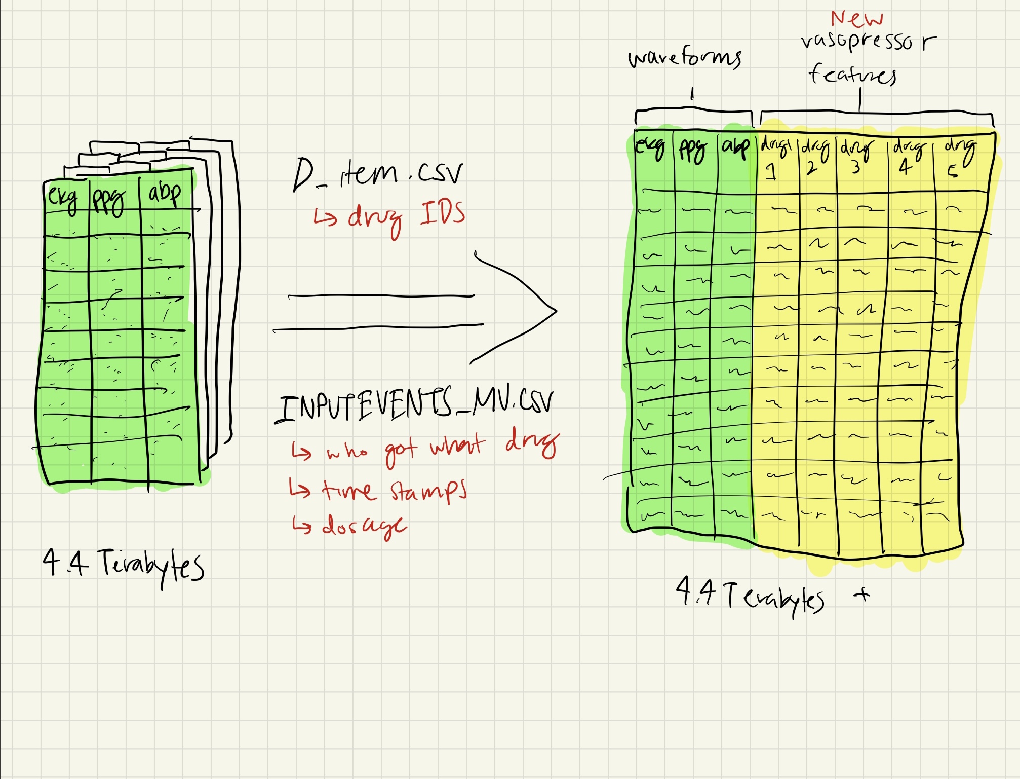
The first step was to scrape the EHR for this vasopressor information. The five vasopressors we looked at specifically were: Epinephrine, Dobutamine, Dopamine, Phenylephrine, and Norepinephrine. However, part of the challenge was finding out which code that was associated with which drug. In the healthcare industry, most items were masked with a numerical ID for privacy reasons. The first step was therefore going through “D_items.csv “to extract the five numerical IDs. Next, we needed to look through “INPUTEVENTS_MV.csv “which contained which patients got what drug, the timestamps of administration, the end timestamp of administration, and the dosage of the vasopressor.
1
2
3

df = df.loc[df['ITEM_ID'].isin(drug_ID)]
Through running this simple one line of code, I could filter out all the patients who didn’t receive vasopressor drugs and/or were not administered the five drugs named. Once we had the filtered CSV file, we saved it and proceeded to write in the drug columns.
Creating new Drug Columns
Writing in the drug columns was the biggest hardship I faced and took nearly three out of the eight weeks of my internship. Because each patient’s EKG, PPG, was being tracked through milliseconds, this resulted in files of upwards to 100 million rows by six columns. The worst part was that we would be adding five columns for each unique vasopressor, which would only increase the file size. Right before I was about to generate these new data files, I checked the data size of our dataset. I was astonished that our dataset came out to 4.4 Terabyte of data even while compressed. Therefore we needed a clever solution to write out these new drug columns.
One of the most valuable skills I was taught this summer was how to run code in parallel. And since the “halperingpu “had up to 80 CPU cores, I was allowed to use up to 20 of them. In addition, I became inspired by the TV show “Silicon Valley,” where they make an optimized compression algorithm called mid-out. Similarly, I was going to start with the first and last patients’ data files and meet in the middle. A visual is displayed below:
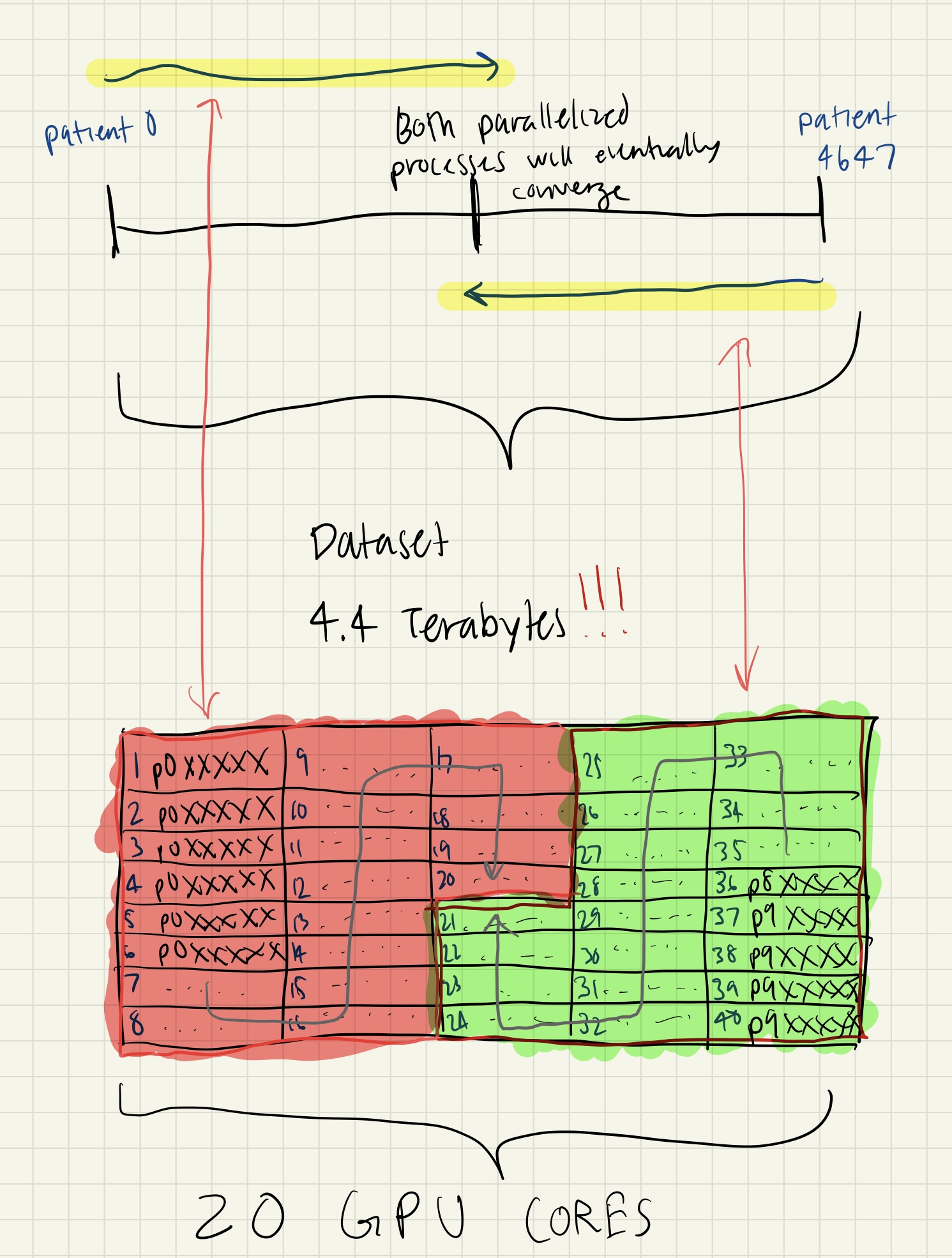
The significant idea was that if I could write out the drug columns and save that entry within a “lockfile.lock “, we could keep the progress of which files have been written into and which have not. Therefore using this Silicon valley inspired parallelized function, I executed this brutal task. And it still took nearly two weeks until it was finished… The code is shown below:
1
2
3
4
5
6
7
8
9
10
11
12
13
14
15
16
17
18
19
20
21
22
23
24
25
26
27
28
29
30
31
32
33
34
35
36
37
38
39
40
41
42
43
44
45
46
47
48
49
50
51
52
53
54
55
56
57
58
59
60
61
62
63
64
65
66
67
68
69
70
71
72
73
74
75
76
77
78
79
80
81
82

def time_calculator(start, end, drug_amt):
   '''
   calculates the end and start time of the patient's drug administration
   and calculates the rate at which the drug is administered
   '''
   d1 = datetime.strptime(end, "%Y-%m-%d %H:%M:%S")
   d2 = datetime.strptime(start, "%Y-%m-%d %H:%M:%S")

   difference = d1.timestamp() - d2.timestamp()
   rate = drug_amt/float(difference * 1000)

   return rate

def write_files(file):

   df = pd.read_csv('/data2/mimic/ABP_with_Med_data/mg/mg_INPUTEVENTS_MV.csv.gz', compression='gzip')
   fileID = file[:18]
   print(fileID)

   l = []
   for i in os.listdir('/data2/mimic/ABP_with_Med_data/patients/flags'):
       i = i[:18]
       l.append(i)

   if fileID not in l:
       print("skipped")
       return 0

   df = df.loc[df['date+ID'].isin([fileID])]
   #display(df)
   print("found something")
   df = df.reset_index()
   df_out = pd.read_csv('/data2/mimic/ABP_with_Med_data/patients/' + file ,compression='gzip')
   print("read in wave file")
   try:
       for i in range(len(df)):
           s = df['STARTTIME'].at[i]
           st = df['ENDTIME'].at[i]
           amount = df['AMOUNT'].at[i]
           rate = time_calculator(s, st, amount)
           print(rate)
           value = s+'.000'
           value2 = st+'.000'
           beg = (df_out[df_out['Unnamed: 0.1'] == value].index.values)
           end = (df_out[df_out['Unnamed: 0.1'] == value2].index.values)
           if rate == 0:
               continue
           # insert drug info to right column
           if df['ITEMID'][i] == 221906:
               df_out['Norepinephrine'][beg[0]:end[0]] = rate
           elif df['ITEMID'][i] == 221749:
               df_out['Phenylephrine'][beg[0]:end[0]] = rate
           elif df['ITEMID'][i] == 221662:
               df_out['Dopamine'][beg[0]:end[0]] = rate
           elif df['ITEMID'][i] == 221653:
               df_out['Dobutamine'][beg[0]:end[0]] = rate
           elif df['ITEMID'][i] == 221289:
               df_out['Epinephrine'][beg[0]:end[0]] = rate
           else:
               continue
           print("columns have successfully been put in")
           if len(df) >= 2 and i % 2 ==0:
               df_out.to_csv('/data2/mimic/ABP_with_Med_data/patients/' + file ,compression='gzip')
               print("file successfully wrote out")
       os.remove('/data2/mimic/ABP_with_Med_data/patients/flags/' + fileID + '.txt')
       return 1
   except IndexError:
       print("something failed")
       os.remove('/data2/mimic/ABP_with_Med_data/patients/flags/' + fileID + '.txt')
       return 0


if __name__ == "__main__":
   l = []
   for i in os.listdir('/data2/mimic/ABP_with_Med_data/patients'):
       l.append(i)
   os.chdir('/data2/mimic/ABP_with_Med_data/patients')

   with Pool(6) as executor:
       results = executor.map(write_files, l)
Retrain model
The last part of my summer was to retrain the imputer model with the new data I had generated. Everything was essentially written within “abp_imputer.ipynb “and all I had to do was change the “git_configs.py “and “abp_model.py “files so that it took in the correct amount of additional channels within our one-dimensional waveform. However, due to time constraints, I could not test the 4000+ patient files I generated in the summer. We couldn’t find a way to load all the data, and training would have taken an extremely long time if I had trained on the whole patient sample. Therefore Dr. Akos Rudas and Dr. Jeffrey Chiang are currently working on those two aspects that I could not. We hope to release a published paper after its completion.
Results
In this section, we take a look at the results generated by the imputer pipeline.
Regression-based Predictions
Our first set of plots shows three different 4-second frames containing the actual waveform, the predicted waveform without the medication, and the predicted waveform with the medication. Though these are just random samples, we can see that both models tend to show off pretty quality-level results.
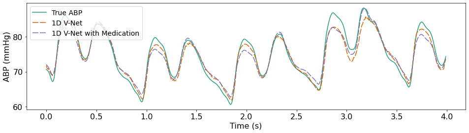
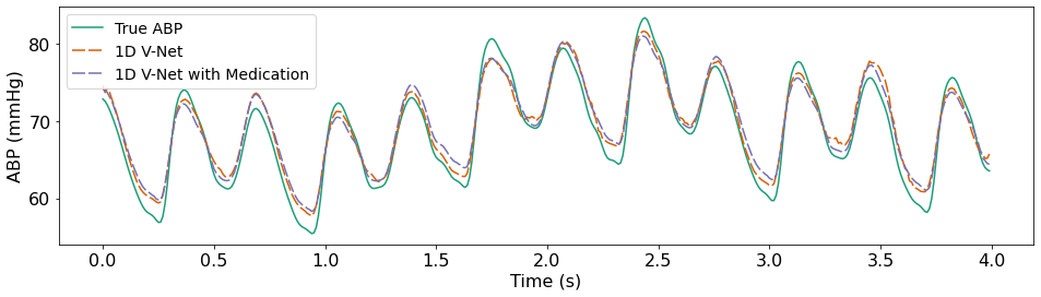
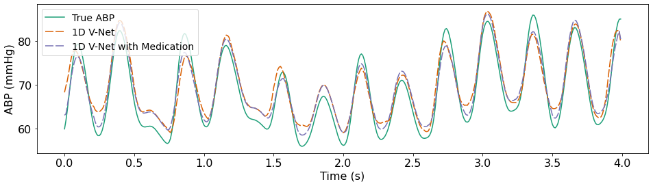
We see the differentiation between the first model and our current model, which considers clinical interventions. Each particular frame is a relatively close race in determining which prediction is doing better. Therefore we need a better-suited test to identify our results.
Bland–Altman
To verify that this model is within the gold standard of invasive blood pressure measurements, we use a method known as the Bland Altman. This Bland-Altman method is the standard for comparing two medical device agreements. Accuracy and precision of the predictions were described as the mean ± standard deviation of the differences between the predicted and true blood pressure values. The Association for the Advancement of Medical Instrumentation (AAMI) criteria considers the differences acceptable if less than five ± eight mmHg. For each four-second window under consideration, we use the peak finding algorithm within our “ABP_imputer.ipynb “pipeline to find the systolic and diastolic blood pressure measurements of our ABP waveform. These measurements can then be used as the standard reference values we can compare within our model. We then use the peak finding algorithm on our predicted waveforms to similarly get a set of predicted systolic and diastolic points and compare these to our reference waveforms. By taking the local alignment by minimizing the sum of differences between indices, we could see the difference between the true and predicted. These plots aim to have a wide distribution of our data centered around the zero line, meaning it is widely accurate across a wide range of blood pressure measurements.
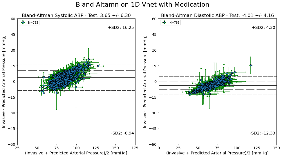
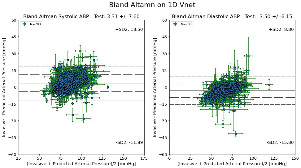
Based on our data, we can see that our model does tend to be performing better, but it also contains bias. This bias, from my understanding, is that we only took into account specific clinical interventions (vasopressors), which would only improve the predictions based on the lower blood pressure. Therefore we can see that the variability is much greater at higher blood pressures, causing a diagonal distribution. Meanwhile, we can see that the original model had no such relationship and was just widely variable. It is safe to say that the predictions on this small subset of data are only small implications, and I look forward to seeing the results of the 4000+ patient model currently in the works.
Code
The code is not publicly available between the Collaborators and me for privacy reasons. Our future hope is that we do publish the code along with the new paper.
Collaborators
SIMON LEE1, Ákos Rudas2, & Jeffrey N. Chiang2 1 Bruins in Genomics Summer Program, Institute for Quantitative and Computational Biosciences, UCLA 2 Department of Computational Medicine, University of California, Los Angeles, CA, USA