Abstract
The Fermi-Pasta-Ulam-Tsingou problem in physics is an apparent paradox that given a system of point masses connected by springs, it will almost exactly form the same periodic behavior known as the Fermi-Pasta-Ulam-Tsingou recurrence, rather than an expected ergodic behavior. This behavior surprised them because they expected the system to thermalize or reach thermal equilibrium in just a short time. However, the system appears to evade the ergodic hypothesis, and this explanation remains a hot topic in research today. Therefore, in this project, we are building a numerical analysis program that will help us visualize linear and nonlinear forms of the Fermi-Pasta-Ulam-Tsingou problem to help us visualize this unique behavior.
Keywords:
Physics simulation, Quasilinear system, Scientific Computing, Fortran
History
In the summer of 1953, Enrico Fermi, John Pasta, Stanislaw Ulam, and Mary Tsingou conducted computer simulations of a vibrating string that included a nonlinear term (quadratic in one test, cubic in another, and a piecewise linear approximation to a cubic in a third). They found that the system’s behavior differed from what intuition would have led them to expect. Fermi thought that after many iterations, the system would exhibit thermalization, an ergodic behavior in which the influence of the initial modes of vibration fade, and the system becomes more or less random, with all modes excited more or less equally. Instead, the system exhibited a very complicated quasi-periodic behavior. They published their results in a Los Alamos technical report in 1955. (Enrico Fermi died in 1954, and so this technical report was published after Fermi’s death.)
Governing Differential Equations
\[ \ddot{x} = f_{i} = K(x_{i+1}-2x_{i}+x_{i-1})(1+\alpha(x_{i+1}-x_{i-1}))\] \[ x_{i}(0) = x_{i}^{0} \] \[ \dot{x} _{i}(0) = v_{i}^{0}\]
In equation 1, \(K\) is the spring constant, \( \alpha \) is the strength of the nonlinearity, and \( x_{i}(t)\) is the deviation of the \(i^{th} \) mass from its equilibrium position. Additionally \( x_{i}^{0} \) is the initial displacement of the \(i^{th}\) mass, and \(v_{i}^{0}\) is the initial velocity of the \(i^{th}\) mass. We assume that all masses are normalized to one. These parameters and this system work for infinite systems of point masses. However, we can determine the size of the system and truncate that system to \(N\) total masses, so \(i=1,…, N\)
In order to solve this particular equation, second order ODE, we must find a numerical method to solve this. Since computers do not perform calculus, methods are constructed to help solve these with computation. Therefore in order to advance solutions through time we are able to take the \( x^{n}_{i} \text{and} x^{n-1}_{i} \) in order to get the next solution. This mechanism is what we call the leapfrog method because we use previous and current solutions to generate a future solution. This solution can be calculated using the following:
\[ {x}^{n+1}_{i} = f_{i} = K(x_{i+1}-2x_{i}+x_{i-1})(1+\alpha(x_{i+1}-x_{i-1})) \]
It is essential to know that this equation, which resembles how we advance our solutions through time, has linear and nonlinear components. In the linear component, we set our \(\alpha\) to be equal to 0. Doing so will have a normal behavior where the mass string oscillates up and down without any surprises.
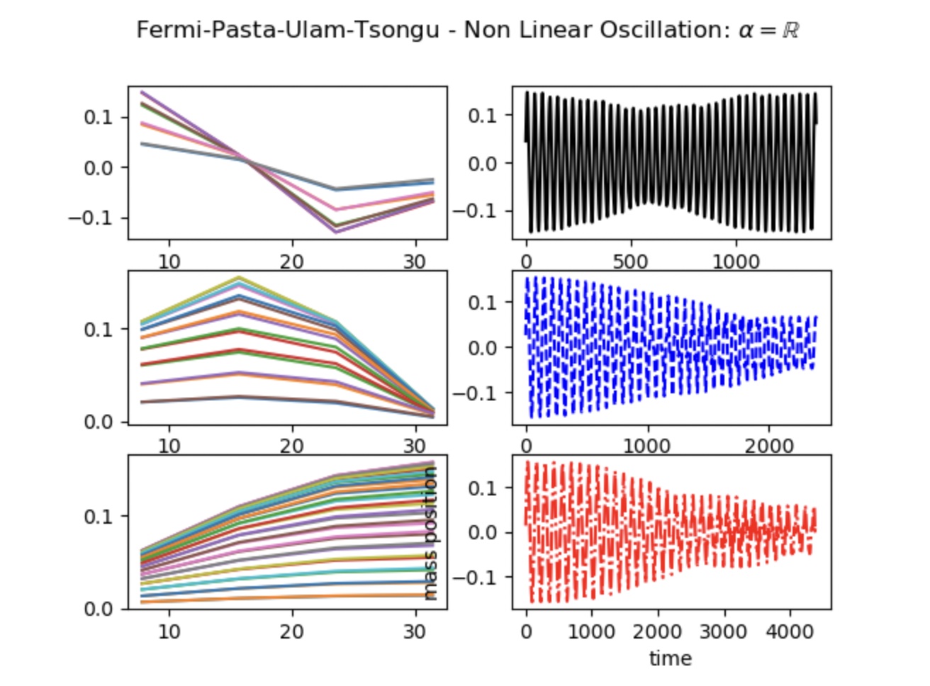
Nothing is obsolete about this behavior; as long as our equation stays linear, the behavior of the masses on a string will remain consistent. However let’s revisit if we include an \( \alpha \) value that is not equal to 0. As mentioned in the Preface, Fermi, Pasta, Ulam, and Tsingou thought the behavior would not follow any pattern. However, as they ran the simulation, they were shocked to find that there was a pattern within this nonlinear system. Why this occurs remains an active part of the research. However, it is odd but amazing how this system, in particular, behaves.
The Simulation
Source Code
code/fortran/Makefile: file that compiles and builds Fortran files
code/fortran/fput.f90: main module that brings together the rest of the files
code/fortran/leapfrog_module.f90: the leapfrog method is contained here
code/fortran/output_module.f90: generates the output files that we used to graph our behavior
code/fortran/setup_module.f90: file that contains setup parameters
code/PyRun/fput_viz.py: file that plots our results
code/fputPrototype.py: the simulation file
Tutorial on how to run code
- run the python file
cd code/PyRun/ | python3 fput_viz.py