Mini Project 3: Glove Sensor Regression
Keywords
Kinematics, EMG, Accelerometer Data, Glove position tracking, Neuroprosthetics, Regression
Introduction
Predicting finger movements using forearm data is a big challenge in neuroprosthetics [1][2]. To this end, various clinical datasets have been published, enabling researchers to develop novel prosthetic hand control techniques. However, existing work has focused on deep learning methods with the goal of predicting intended movement classes [3][4]. These models do not scale well because each new movement class has to be an explicit part of the model’s training set. Therefore, our aim is to investigate whether the exact position of the hand and all digits can be regressed from forearm sensors - EMG and accelerometer data - in real time and whether this learning paradigm can be generalised to novel movements.
Methods
We used three single-subject data acquisitions (Acq.) from the NinaPro 8 dataset. Each Acq. consisted of 9 distinct movements repeated a number of times. Our input data consisted of 16 EMG sensors placed on the forearm and 48 accelerometer (ACC) channels corresponding to the three spatial dimensions for each EMG sensor. The ground truth consisted of 18 position trackers recorded with a dataglove. We performed fundamental data analysis by plotting all data on a time-value axis. We checked the data for outlier signals and missing values, concluding that all channels were suitable. We used the amplitude of EMG data, and all further data processing was done separately for each movement repetition to avoid possible movement artefacts caused by discontinuities between repetition Acqs.
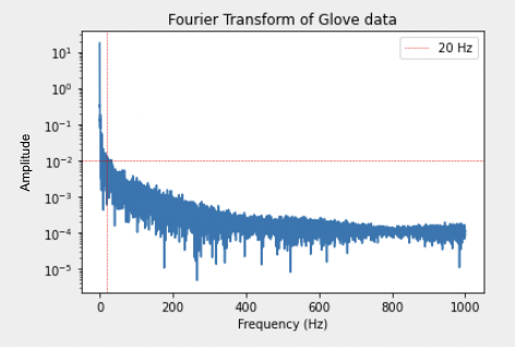
To turn raw time-series data into aggregate data suitable for supervised learning, we selected 50 equidistant sampling windows from each movement repetition. We performed Fourier analysis on each data glove tracker to assess the existence of transient, high-frequency position signals and estimate a valid lower bound for the sample window length. We then considered the practical implications of the window length and selected an intuitive value for the upper bound. We extracted 17 time, frequency, and time-frequency features from each EMG and ACC channel for every window. We then defined label data as the position channels at the end of each window. After normalising the data using their individual min-max intervals, we noticed that a different subset of features per channel produced invalid values. We further explored the root cause of these NaN values, which was the incorrect mapping of constant features to inf values. We corrected these values to 0.5, which preserves all information without the need to drop feature columns.
For the supervised learning problem, we used the XGBRegressor algorithm, which is part of the XGBoost library[5]. Using SKlearn’s GridsearchCV on a subset of the training data (only acq. 1), we optimised the learning rate, max tree depth, and the number of estimators. Window and feature selection were done by training and testing on a 9:1 split of Acq. 1 data, including all movement classes in the training and test sets. The optimal window duration was selected by computing the average relative root mean squared error (relRMSE) across all channels. We performed feature selection using mutual information and imposing a minimum selection threshold. The optimal threshold of the feature score was computed using the RMSE.
Following this, we used the selected parameters to train the model with the complete dataset. Training was conducted on all movements from Acq. 1 and 2, and testing was done on all movements from Acq. 3. To assess whether the model could generalise to novel movement classes, a new round of training was conducted on movements 1-8 from Acq. 1 and 2, and testing was done on movement 9 from Acq. 3. Finally, we investigated the effect of adding previous position data as features. Specifically, the true recordings of all finger position data from the last 3 time points were appended to the feature set. Training was conducted on all movements from Acq. 1 and 2, and the test was performed on all movements from Acq. 3, using true kinematic data as features. The feature importance of kinematic data was then assessed. Considering that ground truth data would not be available at any time point in a practical scenario, a second test was performed by replacing true kinematic test data with the last three instances of predicted tracker positions.
Results
Given that the Fourier amplitude was consistently below 0.01 after 20 Hz (Fig. A), we selected a lower window length bound of 50ms and a practically viable upper bound of 200ms.
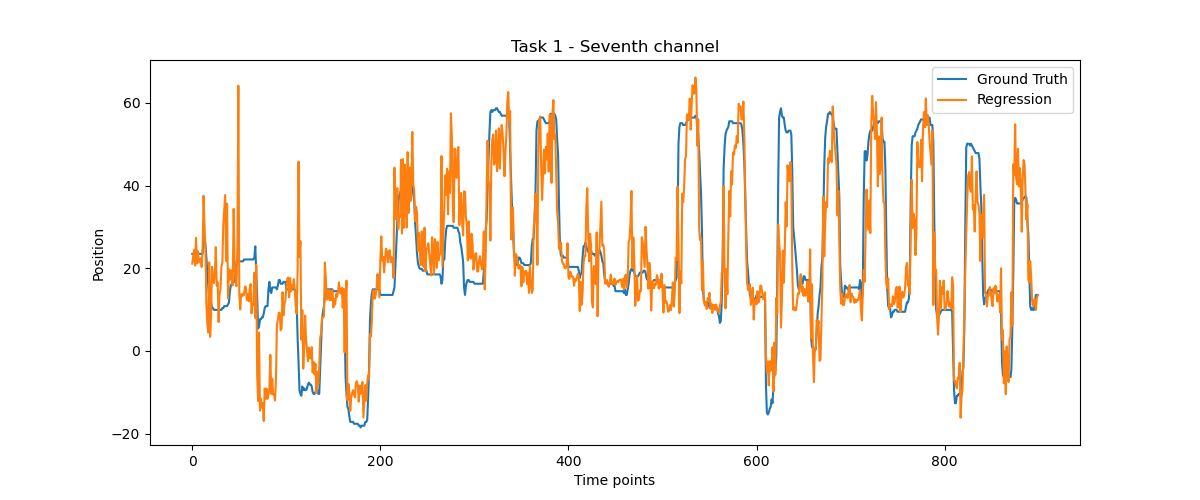
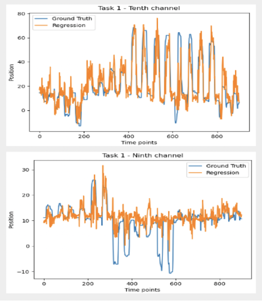
We found that the optimal window length was 150ms, and the associated feature score threshold was 0.3. Test set evaluation (Fig. B) produced an average normalised RMSE (normRMSE) of 0.17 across all channels.
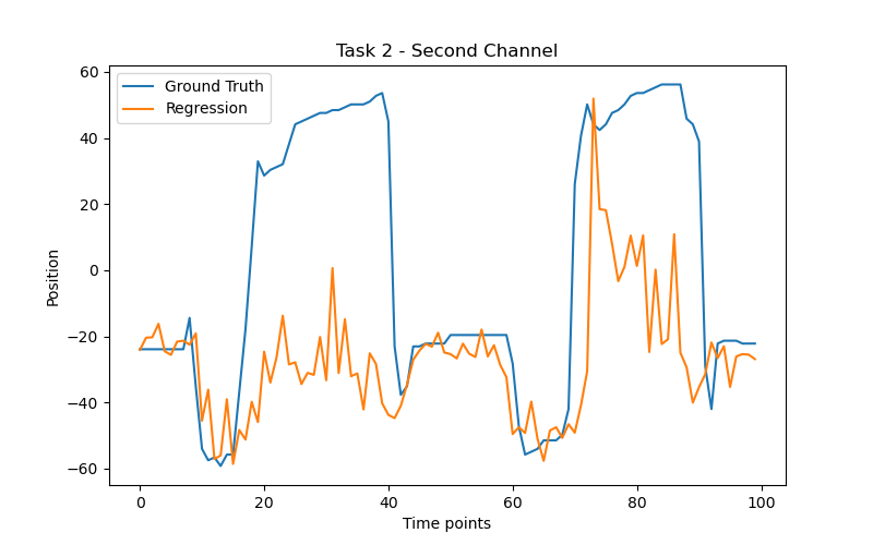
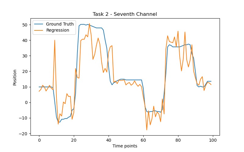
However, when the tested movement was not part of the training set (Fig. C), performance dropped with an average normRMSE of 0.4. We also noticed a higher variation in individual channel performance.
The addition of true past kinematic data resulted in a near-perfect fit (Fig. D), reflected by an average normRMSE of 0.03 This increase in performance is reflected in the importance of the added features, shown in (Fig. D.1)
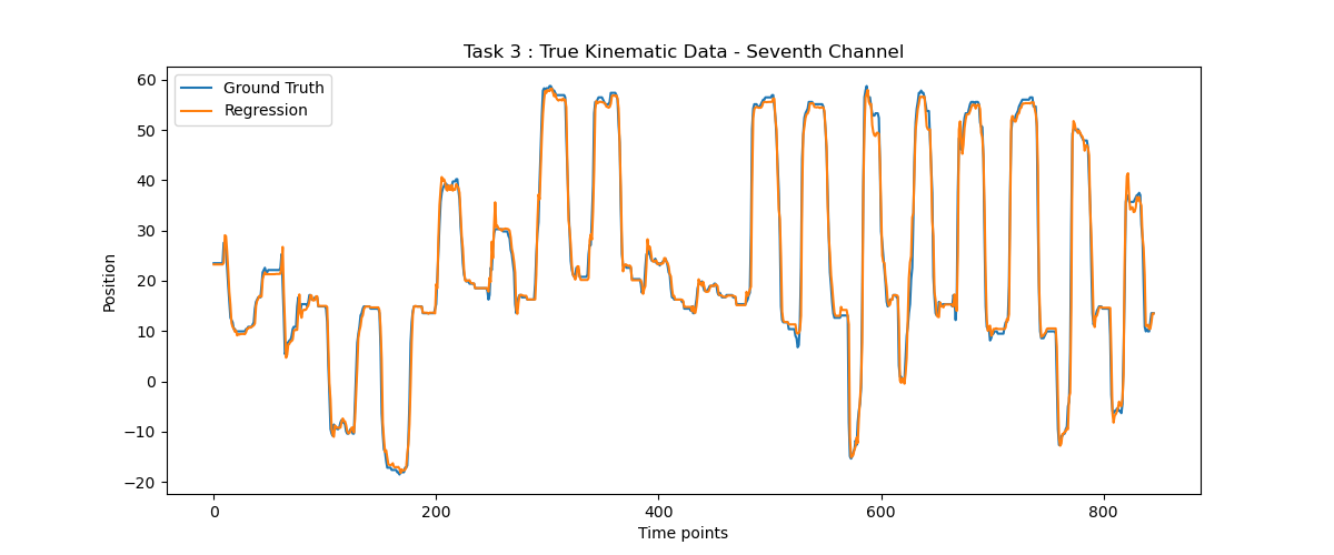
Nevertheless, when true kinematic data were replaced with the last 3 regressed positions (Fig. E), model performance dropped severely, with an average normRMSE of 0.26.
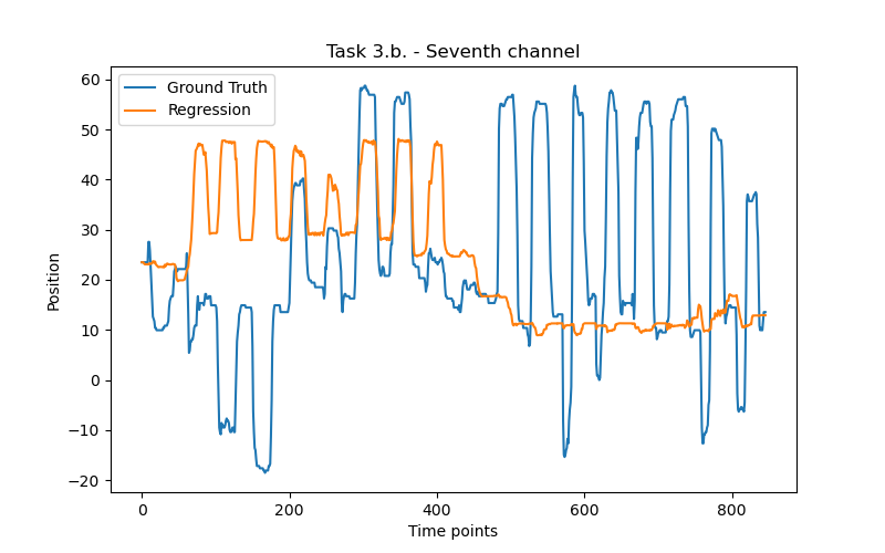
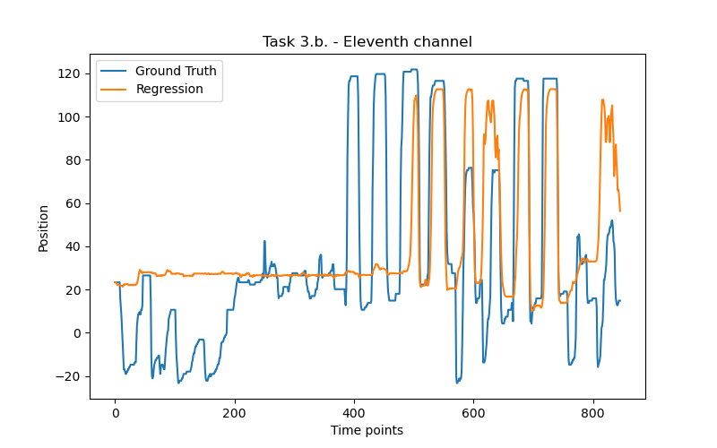
When comparing the results from different channels (Fig. F) we noticed that the performance across them varied the most when predicting novel movements. More specifically, the model performed poorly when dealing with rare and sudden movements versus recurring and oscillatory movements.
Discussion
In our analysis, we used raw time series data to extract relevant aggregate features. Using sample windows meant that subsampling or smoothing was not necessary, as it is already done implicitly through the feature extraction process. Using relative RMSE to select the optimal window length ensured that the homogeneity of performance across channels was taken into account. The relatively large optimal window justifies our argument that transient effects do not exist, and therefore do not need to be captured by smaller windows.
Initial model testing results suggest that EMG and ACC data from the forearm are adequate for training models capable of regressing hand position. However, it seems that training on a vast number of different movements is necessary for the model to generalise well to novel hand movements. This is detrimental to our initial hypothesis that exact position regression could prove a better alternative than movement classification for practical applications. Additionally, while the addition of true kinematic data produces wildly positive results, this performance is unattainable when working with real amputees, as no true hand position would be available. Although these results are disappointing, they are expected given that forecasting long movements without the underlying ground truth is heavily sensitive to divergence. It should be noted that time-series forecasting paradigms exist, which attempt to alleviate the lack of ground truth data by interleaving training and testing sessions. However, these techniques are beyond the scope of standard regression analysis, and they nevertheless require the existence of some ground truth data during training, which makes them potentially not applicable to amputees. Another point of interest comes from the poor results when observing channels with sudden, uncharacteristic movement, which produces unpredictable spikes. This effect places greater importance on using a bigger set of varied movements, in order to introduce intra-channel variation. Nevertheless, it remains to be seen whether the presented model can scale to more movement classes, or whether an upper bound of performance exists as the dimensionality of data increases.
References
[1] A. Baraka, H. Shaban, M. Abou El-Nasr, and O. Attallah, “Wearable Accelerometer and sEMG-Based Upper Limb BSN for Tele-Rehabilitation,” Applied Sciences, vol. 9, no. 14, p. 2795, Jul. 2019, doi: 10.3390/app9142795.
[2] A. Fougner, E. Scheme, A. D. C. Chan, K. Englehart and Ø. Stavdahl, “A multi-modal approach for hand motion classification using surface EMG and accelerometers,” 2011 Annual International Conference of the IEEE Engineering in Medicine and Biology Society, 2011, pp. 4247-4250, doi: 10.1109/IEMBS.2011.6091054.
[3] M. Atzori, M. Cognolato, and H. Müller, “Deep Learning with Convolutional Neural Networks Applied to Electromyography Data: A Resource for the Classification of Movements for Prosthetic Hands,” Frontiers in Neurorobotics, vol. 10. Frontiers Media SA, Sep. 07, 2016. doi: 10.3389/fnbot.2016.00009.
[4] W. Geng, Y. Du, W. Jin, W. Wei, Y. Hu, and J. Li, “Gesture recognition by instantaneous surface EMG images,” Scientific Reports, vol. 6, no. 1. Springer Science and Business Media LLC, Nov. 15, 2016. doi: 10.1038/srep36571.
[5] T. Chen and C. Guestrin, “XGBoost,” Proceedings of the 22nd ACM SIGKDD International Conference on Knowledge Discovery and Data Mining. ACM, Aug. 13, 2016. doi: 10.1145/2939672.2939785.
Code
mini_project3/regression_all_acquisistions.ipynb - the notebook that executes the main pipeline
mini_project3/presentation/Project 3 Presentation.pdf - powerpoint presentation in pdf form of our glove tracking kinematic regression results presented at EPFL.
How to run code
Run the program: (1) Jupyter Notebook
- Run the jupyter notebook
regression_all_acquisistions.ipynb
data can be downloaded here.
Mini Project 2: Multivariate Stimulus Processing Across Brain Regions
Keywords
Independent Component Analysis, Multivariate Methods, Seed Connectivity, Functional Connectivity
Introduction
Monitoring brain activity when presented with a stimulus allows us to distinguish areas of high activity. In a previous project, we looked at univariate approaches which perform the analysis at a per voxel basis. However, when generalized to all voxels they become computationally expensive and highly inefficient. Therefore the focus of this project is to take advantage of multivariate methods. In particular, independent component analysis (ICA) will help us investigate which parts of the brain are spatially active across subjects while watching a movie. We expect to see activation in the visual cortex, and in the default mode network (DMN) regions, which should be active during a resting state experiment. Moreover, we expect to visualize activity in the temporal lobes, caused by responses to sounds coming from the MRI apparatus.
Methods
We used preprocessed fMRI data from 60 subjects watching a silent version of ‘Partly Cloudy’, a short animated video supposed to evoke emotional reactions. Functional data was collected with a gradient-echo EPI sequence sensitive to Blood Oxygen Level Dependent (BOLD) contrast in 32 near-axial slices covering the whole brain (EPI factor: 64; TE: 30 ms, flip angle: 90°).TR used was 2 s and the entire movie was 168 TRs (<6 min).
We ran ICA on this dataset. ICA is a popular multivariate approach in neuroscience, especially in fMRI, which restructures a multi-feature dataset via linear transformation into a self-organized set of functional networks. The advantage of this method over other eigendecomposition methods, like principal components analysis (PCA) or partial least squares correlation (PLSC), is that the components produced from the ICA are statistically independent in only one domain (spatial or temporal). Therefore, its strength lies in detecting brain responses while simultaneously denoising the data.
Two key criteria have to be met when using ICA. The first criterion is that the data must be statistically independent and that our data follows a non-Gaussian distribution. The goal ICA is to find a linear transformation of the feature space such that each of the individual new features is mutually independent:
\[ X=[x_{1}, x_{2}…x_{i}]^{T}-> [y_{1}, y_{2},….,y_{i}]^{T}\ where,] \[ y_{i} ⊥ y_{j} \]
To find this we can solve the following equation: \(Y= WX + n \) , where X is the original data, W is the weight matrix (linear transformation between X and Y), n is noise and Y is the transformed data of independent components.This method can be justified by calculating mutual information, which is the measure of mutual dependence between two random variables (entropy - conditional entropy):
| \[ I(X ; Y) = H(X) - H(X | Y) \] |
This statistical test confirms that the new independent feature space \((yi x yj)\) has no mutual information, effectively justifying its independence: \(I(yi ;yj)=0\). Additionally, the mutual information of the new feature space (Y) with the original feature space (X) is the maximal sum of non-gaussianities of the estimates:
\[ I(Y ; X) = max. \]
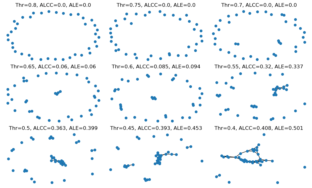
ICA was performed across 60 subjects. Adult (13) and child (47) data were analyzed both together and separately. We investigated three ICA cases with 5, 10, and 20 components respectively. We the performed seed functional connectivity using a brain map of 39 regions. We selected a voxel-seed within the primary visual cortex and a corresponding sphere-seed. Following that, we generated a 39-by-39 functional connectivity matrix, and we produced networks with varying connectivity thresholds, calculating the average local clustering coefficient (ALCC), and the local efficiency (LE).
Results
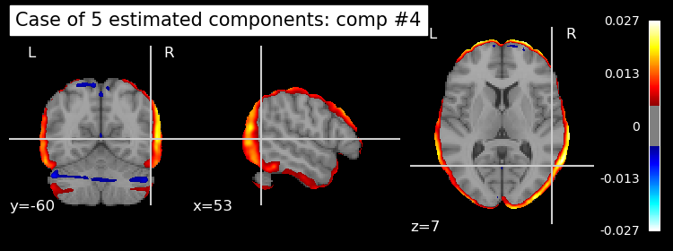
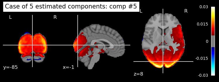
Multivariate Analysis - ICA: In the case of 5-component ICA, individual regions in the brain could not be sufficiently distinguished. The two most meaningful components were the frontal lobe (Fig. 1.a) and the visual cortex (Fig. 1.b). In 10-component ICA, we were able to recognize a number of functional regions that were not present in the previous case, such as the temporal lobes (Fig. 2).
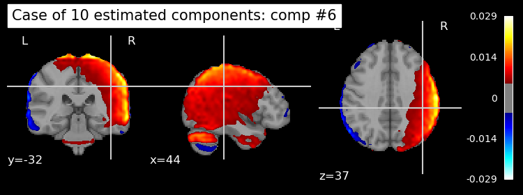
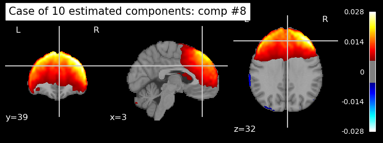
We note that the right (Fig. 2.a) and left (Fig. 2.b) hemispheres were located in different individual components, which could point to preferential sampling of information, proposed by the ‘asymmetric sampling in time’ hypothesis.
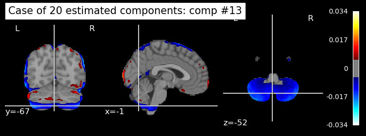
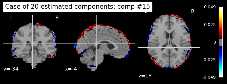
In 20-component ICA, most of the added components were nonspecific “noise” regions (Fig. 3), which did not contribute to our analysis. We also found very high similarity in the individual components of adults and children, indicating that the brain regions involved in the study are already well developed from a young age.
Considering the above findings, we can report three main active regions. The visual cortex, which is the primary site of visual information processing, was present in all ICA analyses. This is in line with our hypothesis and was expected, since the movie-watching task is highly visual. The second active region is the frontal lobe, which contains the prefrontal cortex and is the site where attention and memory are manifested. This is contradictory to our hypothesis, as it means that subjects were attentive and task-positive. It could also offer an explanation as to why the DMN was not present in any of the individual components. The third active region was the temporal lobes, associated with hearing. We must note here that, although some brain regions appear to have negative values, this does not mean that they are less active, but is a product of the mathematical analysis.
Functional Connectivity:
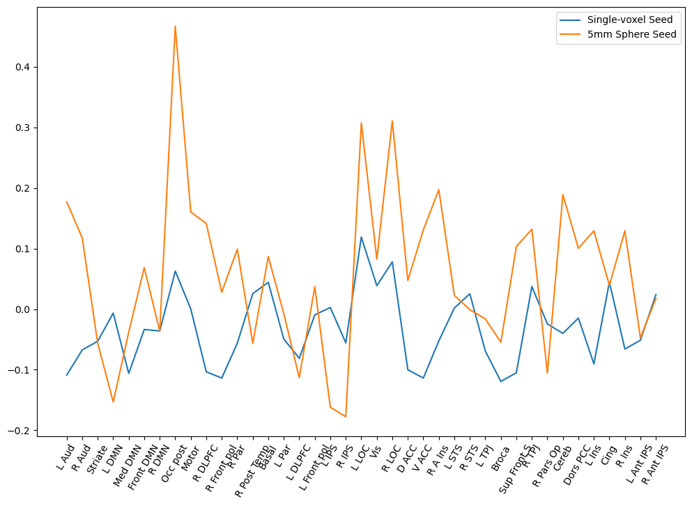
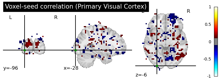
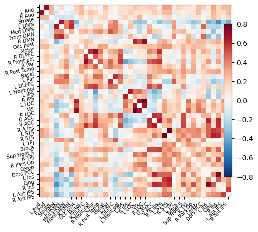
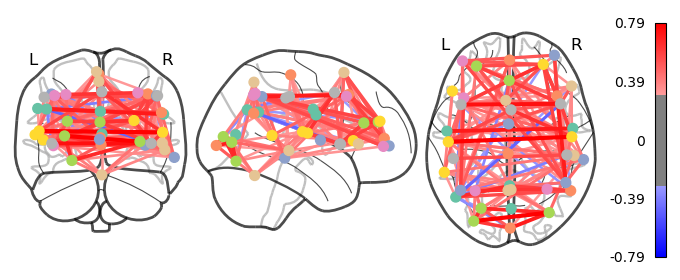
We found that sphere-based seeding performed slightly better in producing high correlations with associated brain regions (Fig. 4). However, single-voxel seeding also produced meaningful correlations, and both methods were able to accurately demarcate the PVC (Fig. 5). The functional connectivity matrix (Fig. 6) is illustrated as a graph in Figure 7. The provided code also offers an interactive view of this graph. Networks with increasing connectivity thresholds and their ALCC and LE metrics are shown in Figure 8. We can observe that none of the networks are fully connected, and a correlation threshold above 0.6 essentially removes all edges.
Discussion - Theoretical Part
ICA is a powerful method, but one of its limitations is finding the correct number of components to obtain the clearest signals. In this project, multiple runs with different numbers of components were needed to get a set of meaningful results (Q1).
The main motivation behind choosing ICA is its strength as a multivariate analysis tool that can work in resting-state conditions, while producing functionally interpretable results. In this case, GLM was ruled out, because it can only be applied to active-condition tasks that can produce meaningful regressors (Q2).
ICA is agnostic to the number of components produced, which must be defined as a hyperparameter. Therefore, it is difficult to find an ideal number of components a priori, as was the case in our project. Even though some components have clear noise characteristics, they are spread out across multiple components and are difficult to confidently rule out. For this reason, other component analysis methods, such as PCA and PSLC, would be better suited for preprocessing GLM data (Q3).
A sphere seed (3D) can be a better alternative to voxel functional activity because it provides a better signal-to-noise ratio. Alternatively, one might use predefined brain atlases to perform functional connectivity, as in the connectivity matrix shown above (Q4).
A graph representation of the brain offers many opportunities for quantitative analyses that wouldn’t be possible through simple contrast visualization. It is a powerful tool to investigate how different brain regions communicate, and it can offer important insights into the overarching architecture of the brain, such as whether the brain follows a centralized architecture, or whether it can be partitioned into distributed functional hubs (Q5).
Footnotes
[1] Vodrahalli, K., Chen, P.-H., Liang, Y., Baldassano, C., Chen, J., Yong, E., Honey, C., Hasson, U., Ramadge, P., Norman, K. A., & Arora, S. “Mapping between fMRI responses to movies and their natural language annotations” NeuroImage 2018 180:223–231
[2] Defining ICA by Mutual Information, http://cis.legacy.ics.tkk.fi/aapo/papers/IJCNN99_tutorialweb/node18.html
[3] Gael Varoquaux, Alexandre Gramfort, Fabian Pedregosa, Vincent Michel, and Bertrand Thirion. Multi-subject dictionary learning to segment an atlas of brain spontaneous activity. In Information Processing in Medical Imaging, 562–573. Berlin, Heidelberg, 2011. Springer Berlin Heidelberg.
[4] Poeppel D. “The analysis of speech in different temporal integration windows: cerebral lateralization as ‘asymmetric sampling in time’” Speech Communication 2003; 41:245-255
Code
mini_project2/ICA.ipynb - the notebook that executes the main pipeline
mini_project2/New - Seed Functional Connectivity & Graph Metrics.ipynb - Extended analysis done for seed functional connectivity and graph based plots
How to run code
Run the program: (1) Jupyter Notebook
- Run the jupyter notebook
ICA.ipynb
New - Seed Functional Connectivity & Graph Metrics.ipynb
Mini Project 1: Processing Faces - Brain Activity Modeling
Motivation
Imagine that we are interested in identifying which region of the brain is involved in processing faces. We can explore this question by showing participants different types of faces where each face represents one trial. If we scanned someone with this design, we could expect to see any region involved in processing faces increase in activation around the time of the face presentation. To understand which of these regions process faces we would need to add at least one other condition/visual stimulus that will serve as a visual control. It’s usually a visual stimulus that has similar properties to a face in terms of luminance and colour. In this mini-project, we’ll see how the general linear model (GLM) can be used to make inferences about brain responses in a single subject. Given the simulated time series for a single voxel that resembles real data, we can evaluate how well we can recover the true signal using a general linear model.
Keywords
General Linear Model (GLM), convolution, signals processing, brain activation
Introduction
Understanding brain functions and their localisation within the nervous system has been a fascination to scientists for a long time and has split opinions throughout history; from René Descartes’ dualistic view of a separate body and mind, Gall’s phrenology all the way to Pierre Flourens’ holistic view.
These turbulent debates were only dissipated thanks to the apparition of magnetic resonance imaging (MRI) used to non-invasively obtain structural images of the brain and functional MRI (fMRI). As neuronal activity triggers increased blood flow in the respective area, detecting the deoxygenated hemoglobin molecules (paramagnetic) gives insight into brain action. The resulting “Blood Oxygenation Level Dependent” (BOLD) signal depends on blood oxygenation, blood volume, and blood flow. Unfortunately, the raw information collected with fMRI is often not easily interpretable due to noise and other brain activity. However, the desired brain activity can be visualised by creating a model linking the input stimulus to the output fMRI data. By fitting the model to the raw data and plotting its weights onto a structural MRI image, it becomes apparent which voxels react strongly to the stimulus, effectively identifying the brain region responsible for a specific process. These technical advancements resulted in the general adoption of the distributed processing view of the brain, in which different areas are responsible for specific tasks, and complex processes result from the interactions between them.
The complex function of interest in this project is the identification of faces. The core system responsible for facial recognition consists of three regions of the occipitotemporal visual extrastriate cortex. The first region is the inferior occipital gyrus and is associated with the perception of structural facial features. The second is the superior temporal sulcus and is related to changeable aspects of faces, such as perception of eye gaze and facial expressions. Finally, the third region is the lateral fusiform gyrus, which participates in identity recognition. In addition, the extended system includes brain regions that do not solely participate in facial recognition but aid the core system by extracting other meaningful information. One example is the amygdala, which, together with the insula, processes the emotional content of faces.
This project will try to understand how to use a general linear model (GLM) to extract information from brain signals. For simplification purposes, we will treat the data from a single voxel.
Methods
In order to acquire a detailed understanding of fMRI and the modeling of the resulting data, we will first build a fake raw fMRI signal and then decode it with a mathematical model. We mimic showing participants images of faces, objects, or nothing with a series of rectangular pulses. The convolution of this input signal with the ideal Hemodynamic Response Function (HRF) gives us the ideal output data. A more realistic representation of this output is achieved by adding normally distributed noise to the HRF before convolution. Since fMRI data quality can easily be ruptured through a series of artefacts, we wanted to add some Gaussian noise to take into account a more genuine experimental design.
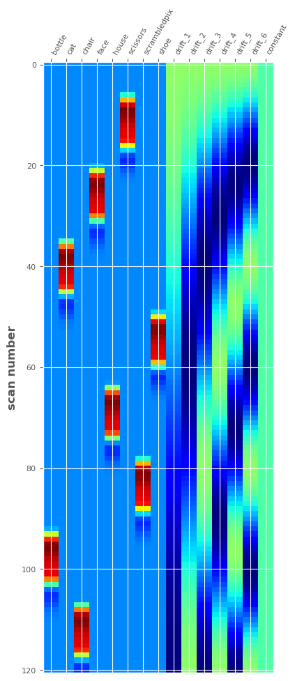
After applying a convolution between our HRF and stimulus signals, we then want to form a design matrix. This design matrix in the context of our problem will be separated into 4 separate columns. Those columns are: faces, objects, noise, and a constant column. The amount of columns we have will be the amount of predictors we will have when we fit our model. This step is important because the amount of predictors would widely affect the precision of fitting an oscillating signal.
After constructing the design matrix, a mathematical model is then fitted to the obtained imitation of raw fMRI data. The modelthat was alluded to was the General Linear Model (GLM), which calculates its weight (\( \beta_{0}, \beta_{1}, … \beta_{n} \)) coefficients by the ordinary least squares (OLS) method, and was fitted with a mean square error cost function. We determine the quality of the fit by testing the optimal weights for statistical significance from the null hypothesis. Below we will display some of our simulations of these processes:
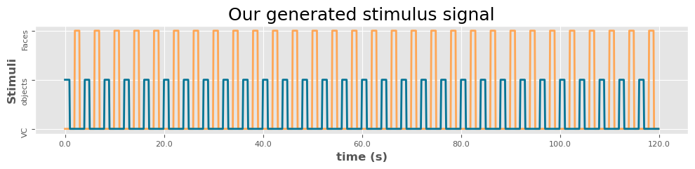
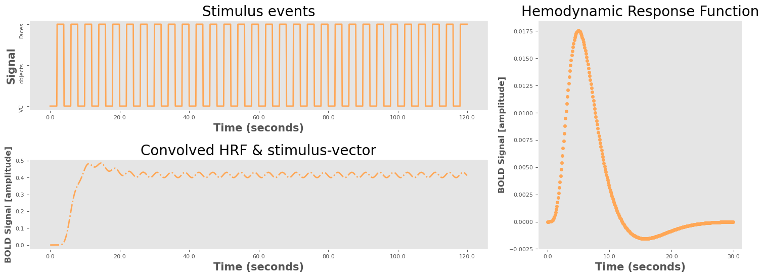
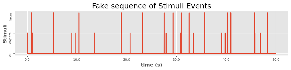
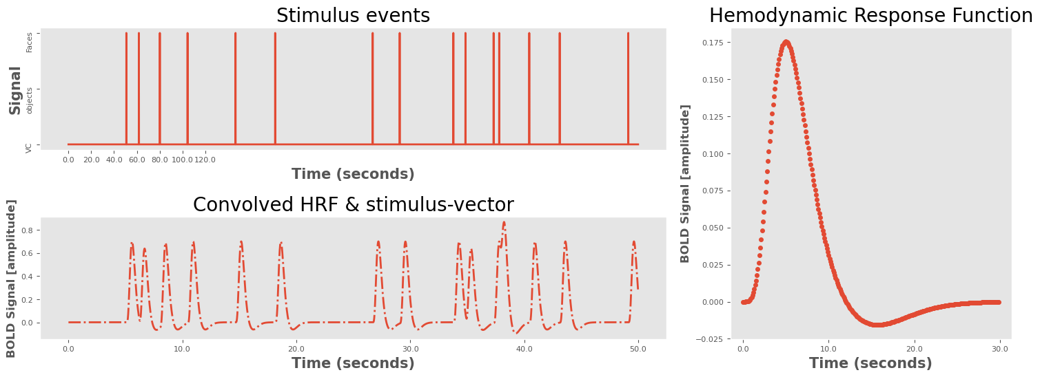
As displayed above we can design a brain voxel experiment with any type of signal. We see that even if the stimuli are instant or are displayed for longer durations that our convolved signal takes a similar form. If we were to add more “rest time” between signals, we would see an oscillating sequence of the hrf function with respect to the amplitude of our signal. So really, we can fit any type of signal through these two steps which we then used as input. After doing so we can produce results of multiple different experiments by constructing the design matrix then fitting it into our GLM.
Results
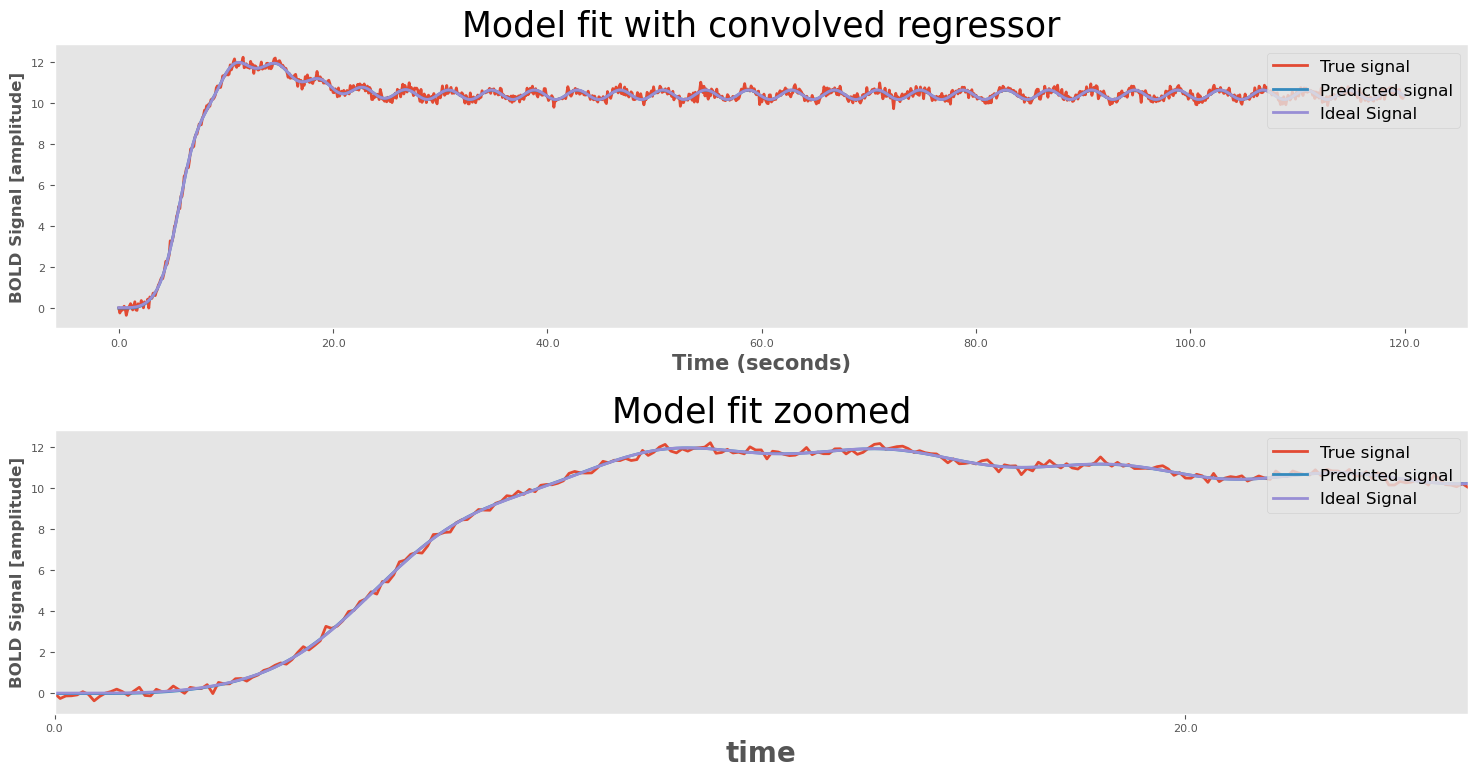
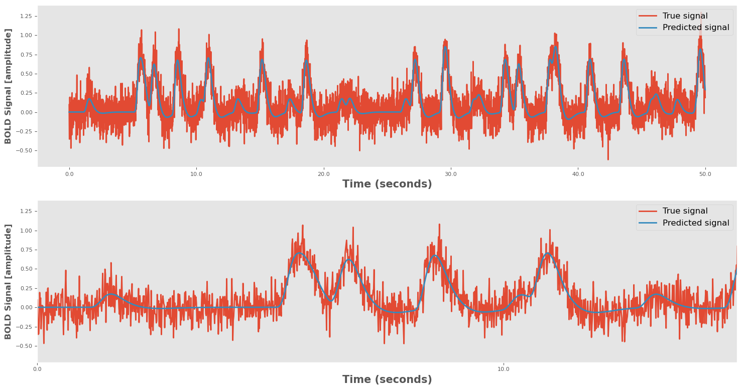
Above we can see our predictions of our one voxel experimental design. The general linear model (GLM) applied to the signal was a good fit with a mean square error of 0.019 for the first experiment compared to the ideal expected output. Another behavior we quickly observed showed the effect of changing the \( \alpha_{1} \) and \( \alpha_{2} \) parameters in our HRF. A high \( \alpha_{1} \) value corresponds to lower amplitude, a slower rise time, and less undershoot. On the other hand, a high \( \alpha_{2} \) value results in an attenuated undershoot that more slowly returns to baseline. So by playing around with our alpha values, we could get some differentiating results.
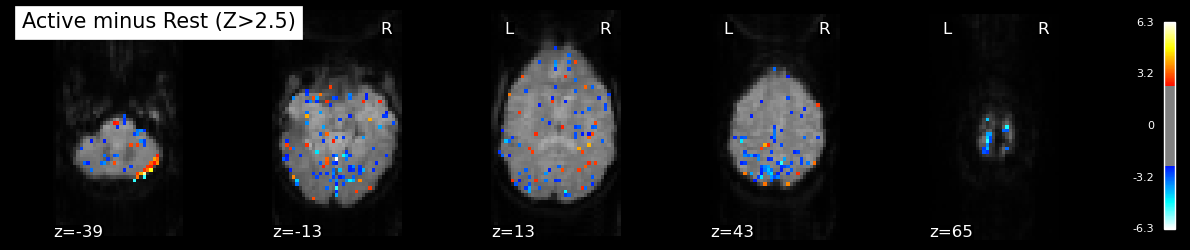
We also fitted our model onto real fMRI images. A one-voxel demonstration would not totally be sufficient to truly explain facial processing brain activity. Similar to our one-voxel signals, we take an fMRI recording that is presented with a series of stimulus events that could monitor brain activity. These images are then captured in the experiment and we could fit these signals (images) onto a GLM model. Using the FSLeyes Python Package which is widely used in Neural Processing, we apply a GLM fit to our data. However unlike our one-dimensional voxel we are able to locate spatially the actual brain activity. The big idea is if we apply OLS on each voxel of the brain, many of our predictors would remain constant in most regions of the brain. However at some important regions disclosed in our introduction like the occipitotemporal visual extrastriate cortex, we can see that those predictors increase or decrease significantly. By applying a mask to our array of predictors, we can also identify what signals are causing what regions to stimulate. We can then take our design matrix and map it to our brain regions that are being activated to see correspondence between the stimuli and the particular brain region. We display some of our results below:
Discussion
This project allowed us to gain insights into experimental design, linear modeling, and the hemodynamic response at the voxel & brain level. We learned that in order to validate our results, we would need to analyze the weights to determine if they are statistically different from the baseline, effectively informing us of their activation during facial recognition. We therefore performed some t-statistic tests: \(t = \beta_{j} / \sigma_{j} \), where \( \beta_{j} \) refers to the estimated parameter for the regressor \(j \) and \( \sigma_{j} \) refers to the standard error of regressor \(j \). We identified that t values that are more than two standard errors away from zero are statistically significant, and therefore we are more confident that the estimate is stable and not just an artefact of a small sample size. (Our Statistics are displayed in our notebook)
On top of that we concluded some other observations through this experimental design. Our first was that by varying the signal amplitude, one varies the signal-to-noise ratio (SNR), as most noise would remain constant. As a result, the model fit would suffer as the estimations would be more difficult due to a higher SNR. Also, noise is additive to the signal, so if we want to design a proper experiment, we should be at least of the same order of magnitude if we still want to extract meaningful information from it. Otherwise, the signals would be entirely be covered by the noise.
Some concluding remarks is the amazing strengths of linear modeling. Our group was astonished to see how well we could predict voxel signals at such incredible precision. Additionally, by applying some high-level packages, we were able to apply this model onto actual fMRI data to gain meaningful information about the spatial locations of brain activity. With the brain being such a really complex structure, we were not surprised to see that multiple locations in the brain were actually activated when presented with particular stimuli. Therefore we come away from this project truly amazed at the power of simple computational algorithms in modeling brain activity.
Code
mini_project1/mini_project_1.ipynb - the notebook that executes the stimulus recognition pipeline
mini_project1/example_voxel_signal.npy - the numpy file containing an example voxel
References
[1] Principles of Neural Science, Sixth Edition, 2021 - McGraw Hill. By Eric R. Kandel, John D. Koester, Sarah H. Mack and Steven A. Siegelbaum.
[2] Human Neural Systems for Face Recognition and Social Communication James V. Haxby, Elizabeth A. Hoffman, and M. Ida Gobbini
[3] https://books.google.it/books?hl=en&lr=&id=G_qdEsDlkp0C&oi=fnd&pg=PA193&dq=experimental+design+number+trials+fMRI&ots=Xn2MByS6SG&sig=CNs2Qq6N0zj9DxKSuPwMnYpTH8c&redir_esc=y#v=onepage&q=experimental%20design%20number%20trials%20fMRI&f=false
Collaborators
- Simon Lee
- Julian Thomas Bär
- Veronika Calati
- Merkourios Simos