Abstract
Alzheimer’s disease is a common neurodegenerative brain disorder that slowly deteriorates our cognitive abilities (thinking, memory, and carrying out simple tasks). Alzheimer’s disease has been known to have an unpredictable onset and is, therefore, hard to detect in its early stages. Therefore, there is currently much interest in applying deep learning models to learn from MRI images for early diagnosis. Using publicly available data from Alzheimer’s Disease Neuroimaging Initiative (ADNI), we train an optimized Convolutional Neural Network (CNN) model to predict whether a patient has Alzheimer’s through the features in an image. With high accuracy, we believe our optimized model can have an impact in the medical field and assist medical professionals and researchers in advancing pathology- related tasks. Building these prediction-based models can improve diagnostic accuracy, optimize patient care, and reduce costs by bringing global collaborations.
Keywords
Alzheimer’s Disease (AD), Convolutional Neural Networks, Computational Pathology, Deep Learning
Motivation
Alzheimer’s Disease (AD) is a progressive neurodegenerative condition that leads to short-term memory loss, dementia, and many other cognitive-related issues. These effects are commonly mistaken for stress or aging and often go unnoticed. However, by the time health professionals do detect Alzheimer’s, it is often too late. For a disease that affects every 1 in 9 (11.3%) people ages 65 and older in the United States, this has become a relatively large-scale issue. Traditional methods of diagnosing Alzheimer’s, including a mixture of cognitive tests and brain scans, have been complex markers to track this progression, leaving health professionals stuck. However, in today’s age of data, innovative approaches like machine learning have helped propel not only the field of pathology but the world. Therefore this research aims to build an image analysis computational framework that will allow for the early detection of AD.
To solve this problem, we need to leverage innovative approaches such as machine learning, which are computationally intensive and non-traditional in the medical field. However, machine learning techniques have been increasingly used in disease prediction and visualization to offer prescient and customized prescriptions. Physicians and medical specialists sometimes are left with tough decision-making and fear the extreme penalty of misdiagnosing a patient. So by taking these computational approaches, we not only im- prove the patients’ quality of life, but this also aids physicians in making decisions. With computers showing promise with their high level of precision, this is only the beginning of this partnership between computation and healthcare. This approach aims to identify the knowledge gaps, avoid human error and explore potential opportunities associated with machine learning frameworks.
Deep Learning
Deep learning is a subsection of machine learning methods based on neural networks, which have the power to learn based on representation (Schulz et al., 2012). These models learn very similarly to humans by mimicking how neurons signal and communicate from one to the next. Deep learning is especially important in image analysis because images contain a lot of features (shape, color histogram, color contrast, texture, etc.). When working with such high dimensional data, a simple machine learning model will struggle to interpret and return valuable data for us to analyze. In contrast, deep learning models can process many features, making them very powerful in dealing with image data. So through the deep learning algorithm called the Convolutional Neural Network, we intend to be able to accurately predict whether a patient has Alzheimer’s disease from a set of images. In the preceding sections, we will lay out the foundation and the underlying background knowledge required to understand how we obtained our results.
Data Availability
Data used in this work were downloaded from the ADNI database run by the Laboratory of NeuroImaging at the University of Southern California. The ADNI is an ongoing, longitudinal study designed to develop clinical, imaging, genetic, and biochemical biomarkers for the early detection and tracking of AD through Magnetic Resonance Imaging (MRI) scans. We, therefore, use the complete ADNI1 1yr 3T dataset, which contains 58 AD MRI scans, 113 controlled (CN) MRI scans, and 133 Mild Cognitive Impairment (MCI) MRI scans for a total of 304 complete 3D brain images. The 3T MRI scan is twice as strong as a standard 1.5T MRI. It operates at a strength of 3T; Tesla (T) is the measurement unit indicating a magnetic field’s strength. A stronger magnetic field provides more detailed images, helping doctors and radiologists see more structures inside the body (Duggan-Jahns et al., 2013). For this reason, we also use this magnetic strength to get the most explicit images for our image analysis.
Model
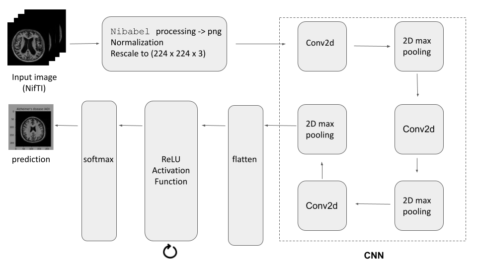
We begin explaining the model we will use to train for accurate prediction. As seen in the above figure, we can see that a lot is going on before we reach our prediction stage. Therefore in the preceding subsubsections, we will break down the processes within our CNN model.
Preprocessing
Pre-processing is one of the most critical steps in machine learning, especially in computational biology (Chicco et al., 2017). Data preprocessing is the manipulation and dropping of data to ensure/enhance the model’s performance. Often if preprocessing is not involved, it can lead to misleading results. Especially in medical images, preprocessing is an essential step because we often get varying levels of quality. It is important to run some cleanup on our data before feeding it into our model.
One of the first significant steps during the preprocessing was to convert our MRI scans from the NifTI (.nii) format into the png lossless image format. Therefore, we used a python script from (OfStack et al., 2021) to perform this conversion for us. By performing this critical step, we significantly reduce our dataset from 11.94 Gb to 52.10 Mb, which is a 99.60 \% compression rate. We hope that through this size reduction, our model can handle all the data on memory and be trained optimally by not having to feed such a large amount of data during our training process.
In addition to our file format conversion, we normalized our image data because some MRI scans have varying qualities. Neural networks process inputs using small weight values, and inputs with large integer values can disrupt or slow the learning process (Brownlee et al., 2019). As such, it is good practice to normalize the pixel values so that each value has a value between 0 and 1. Additionally, we also converted the image’s shape to 224 x 224 x 3, making it really easy to feed into our Convolutional Neural Network with no varying sizes. Our data can be visualized as seen in the below figure.
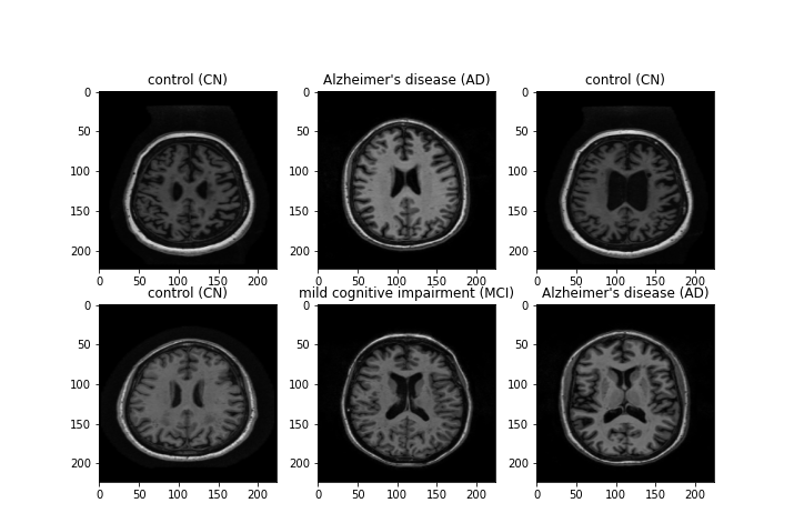
Lastly, as part of the preprocessing step, we split our images into testing, validation, and training sets. We manually performed this split and came to the following breakdown: 1568 images for the training set, 391 images for the validation set, & 419 images for the testing set.
CNN
CNNs are currently the standard for any image analysis problems, and similar works have been done by the following groups (Oh et al. 2019, Folego et al. 2019). A CNN is deemed the perfect type of neural network for these problems because it can successfully capture the Spatial and Temporal dependencies in an image by applying relevant filters. The architecture performs a better fitting to the image dataset due to the reduction in the number of parameters involved and the re-usability of weights. In other words, the network can be trained to understand the image’s sophistication better. The role of the CNN is to significantly reduce the images into a form that is easier to process without losing features critical for getting a good prediction. This is important when we design an architecture that is good at learning features and scalable to massive datasets. Within a CNN, it is made up of two things: a convolution layer and a max pooling layer.
Convolution layer
The 2D convolution layer is the primary building block of CNN (Habibi et al., 2017). It performs a simple operation: we begin with a filter, which is simply a smaller matrix of weight and begins sliding it over the 2d image matrix, and perform an element-wise multiplication on it. This element-wise multiplication is then summed up and stored into a single output pixel.
The filter repeats itself until every location of the 2d matrix is filled. We converted a 2D matrix of features from this convolution filter into a smaller reduced 2d matrix of features. The reduced feature matrix is determined based on the size and shift of the filter.
Let us also consider why this convolution is robust compared to a standard fully connected layer. If we have a network with a 5 × 5 = 25 input features and 3 × 3 = 9 output features. If we were to use a standard fully connected layer, we would have a weight matrix of 25 x 9 = 225 parameters which is too large to consider. Especially with the intensive image file sizes, this would not perform optimally. Therefore, convolution allows us to do this transformation with only 9 parameters. The big idea of convolution is that we do not have to look through all the input features but instead get a general sense of an input feature coming from the exact location. In hindsight, this process is a dimensionality reduction occurring.
Max Pooling
The other significant component of the CNN is the 2d max pooling. A pooling layer is a new layer added after the convolutional layer. Commonly, this pooling happens after the convolutional layer because it helps order layers within a CNN that may be repeated multiple times in a model. It operates separately from our output feature matrix produced by the convolutional layer. It creates a new set of the same number of pooled feature maps.
Pooling involves selecting a pooling operation (average pooling/ maximum pooling), much like a filter applied to our feature matrices. When implementing CNN, the size of the pooling filter is typically a 2 x 2 matrix. This reduces the size of features by at least a factor of 2. In the context of our problem, we have included three maximum 2d poolings that take the maximum value for each patch (pooling filter) of our features matrix.
The main result we get from applying a pooling layer is that the newly produced pooled feature matrix summarizes the features detected within our input. Maximum pooling is partly done to help overfit by providing an abstracted form of our image. Moreover, similarly to the convolution layer, it reduces the computational cost by reducing the number of features to learn from as a form of dimensionality reduction. The pooling outcome is the model’s invariance to local translation (Biscione et al., 2021). So the CNN’s primary purpose after applying a series of convolutional layers and Maximum pooling layers it to get a widely reduced representation of our original image.
Outside layers
Lastly, we wanted to discuss our output layer, which consists of a flattened layer, and seven Rectified Linear Units. (ReLU) activation functions, as well as a softmax before making an informed prediction. Flattening converts our data into a column vector, which will then be inputted into our ReLU activation functions. As part of the output layer, one of the most important aspects is to clean up our reduced data before making a prediction. Therefore the ReLU activation function has become notorious for this post-processing step. Its primary goal is to drown out the negative numbers to zero while not changing the positive input. However, in our case, we take the activation function of different size units meaning that every time we call the ReLU, a new positive integer defining the dimensionality of the output space is produced. After we have iterated through the 7 different ReLU functions, we finish it with a Softmax function, another activation function. At a high level, it predicts a multinomial probability distribution, which calculates a probability between 0 to 1 for that feature. The softmax is used primarily in these multi-class classification problems where class membership is required on more than two class labels. So in the context of our problem, these probabilities will allow us to classify our image into one of three labels: AD, MCI, CN.
Training Parameters
Optimization Function & Loss Function
Lastly, we wanted to describe the optimization function & loss functions we chose to train our model. Machine learning models learn from gradient descent, a process by which we find the local minimums of a differentiable function. It is hard to think that images are differentiable functions, so we can view it more as a method in machine learning that helps us find the values of a function’s parameters (coefficients) that minimize a loss function as far as possible. Therefore we used the Adam Optimization function (Kingma et al., 2014), a stochastic gradient descent algorithm performing exceptionally with images. The method is efficient when working with a significant problem involving many data or parameters. It requires less memory and is highly efficient. Intuitively, it combines the ‘gradient descent with momentum’ algorithm and the ‘RMSP’ algorithm. Combining these two algorithms allows for minimal training cost, which is precisely what is sought in an optimization algorithm.
With our optimization function being explained, we now focus on the loss function we want to minimize. The Sparse Categorical Crossentropy Loss Function is the standard in image processing problems, and the equation can be visualized by the following:
\[ J(w) = - \frac{1}{N} \sum_{i = 1}^{N} [y_{i} log(\hat{y_i}) + (1-y_i)log(\hat{y_i}) ] \]
Let us break down the above equation. \(w\) refers to the model parameters, e.g., neural network weights. \(N\) is the number of parameters of your current model. \(y_{i}\) is the true label, and \(\hat{y_i\) is your predicted label. Its main advantage is its computational cost, which helps us build our CNN. The sparse categorical cross entropy saves time in memory and computation because it simply uses a single integer for a class rather than a whole vector.
Results & Discussion
In our Jupyter notebook script, we have left our last cell to make these predictions. The model can accurately predict all six random images on the validation set. However, running it through our testing set only usually identifies 4 out of the 6 images with an accurate diagnosis. Alzheimer’s disease is brutal to predict, and most machine-learning models used in these studies have tended to have less than 50 % accuracy (Marinescu et al., 2020).
In our discussion, we wanted to highlight some future works. One of the most significant things we want to counter in these pathology problems is to avoid a false negative. A case for a false negative diagnosis would be if a person with undetected Alzheimer’s disease (AD) were predicted to be controlled (CN). This would be detrimental as missing an AD diagnosis can lead to worsening effects as time goes on. Even in our data set, patients were getting at most 3 MRI scans per year, while the average person gets one every 2-5 years. So while we cannot necessarily provide perfect predictions due to unclear disease onset, the least we could do when the model is unsure is to avoid a false negative diagnosis. Regarding doing that computationally, we currently have ideas of making another category in which images could classify. Along with CN, MCI, and AD, we might try to design an architecture where NA could be some uncertain label for predictions. This way, we can further examine these MRI scans using more traditional practices through medical professionals. We would also like to avoid false positives (if a CN patient is predicted to have AD). However, being cautious of these neurodegenerative diseases is not the worst.
Another future work is the application of this model to other diseases. With this recent surge of data, accurate patient data has become one of the more accessible modalities. With all types of researchers trying to understand these more complex diseases, patients have been more willing to give scientists this type of accessibility. Therefore we believe that we could use this same model, change up the labels they could classify, and try running it on other diseases. We hope that once there is more understanding of what physical changes occur in some of these complex diseases, we can highlight those features and use this software to assist medical facilities. Therefore, much excitement is ahead for the medical image analysis field.
Code
“data “- the folder where data generated is stored.
“mri_data_png “- folder containing all the brain scans
“Alz_Predictor.ipynb “- Jupyter notebook to run the CNN Pipeline
alz_model1.h5 - - the machine learning model saved on a h5 file
nii_to_jpg.ipynb - converts NifTi to jpg
How to run code
- Run the notebook
Alz_Predictor.ipynb
References
[1] Schulz, Hannes; Behnke, Sven (1 November 2012). ”Deep Learning”. KI - K ̈unstliche Intelligenz. 26 (4): 357–363. doi:10.1007/s13218-012-0198-z. ISSN 1610-1987. S2CID 220523562.
[2] Duggan-Jahns, Terry (June 24, 2013).” The Evolution of Magnetic Resonance Imaging: 3T MRI in Clinical Applications”. eRADIMAGING.com. eRADIMAGING.com.
[3] Chicco D (December 2017).” Ten quick tips for machine learning in computational biology.” BioData Mining. 10 (35): 35. doi:10.1186/s13040-017-0155-3. PMC 5721660. PMID 29234465.
[4] OfStack (July 22, 2021)” python converts batch nii files into png images.” https://ofstack.com/python/37028/python-converts-batch-nii-files-into-png-images.html
[5] Brownlee Jason (July 5, 2019)” How to Manually Scale Image Pixel Data for Deep Learning” https://machinelearningmastery.com/how-to-manually-scale-image-pixel-data-for-deep-learning/
[6] Oh, K., Chung, YC., Kim, K.W. (2019). “ Classification and Visualization of Alzheimer’s Dis- ease using Volumetric Convolutional Neural Networks and Transfer Learning. Sci Rep 9, 18150. https://doi.org/10.1038/s41598-019-54548-6
[7] Folego, Guilherme, Folego, G., Weiler, M., Casseb, R. F., Pires, R., Rocha, A. (30 Oct. 2020). “Alzheimer’s Disease Detection Through Whole-Brain 3D-CNN MRI.” Frontiers in bioengineering and biotechnology vol. 8 534592. doi:10.3389/fbioe.2020.534592
[8] Habibi, Aghdam, Hamed (2017-05-30). Guide to convolutional neural networks: a practical application to traffic-sign detection and classification. Heravi, Elnaz Jahani. Cham, Switzerland. ISBN 9783319575490. OCLC 987790957.
[9] Biscione, V. and Bowers, J (2021). Convolutional Neural Networks are not invariant to translation, but they can learn to be. https://openreview.net/forum?id=WUTkGqErZ9
[10] Kingma, Diederik P., and Ba, Jimmy (2014) Adam: A Method for Stochastic Optimization. https://arxiv.org/abs/1412.6980
[11] Razvan V. Marinescu, Neil P. Oxtoby, Alexandra L. Young, Esther E. Bron, Arthur W. Toga, Michael W. Weiner, Frederik Barkhof, Nick C. Fox, Stefan Klein, Daniel C. Alexander, (February 2020) TADPOLE Challenge: Results after 1 Year Follow-up. the EuroPOND Consortium. https://arxiv.org/pdf/2002.03419.pdf